Engineering a Lagrangian for Physics, Sensitivity, and Design

44 minute read

Published: October 20, 2026

Consider changing the material thickness distribution of a flexible rotor blade. Such a change affects how much it weighs, how strongly it resists bending and twisting deformations, and how much load it can carry before the material begins to yield. To choose an optimal material thickness distribution that complies with the blade motion, we need to determine the motion it undergoes, the stresses it experiences whilst in motion, and the rates at which these quantities change with the span-wise thickness to minimize cost.

To engineer this blade, we are choosing a thickness distribution that meets a target while satisfying the requirements of its motion and strength. We shall ask a similar question in mathematics: how do we engineer a scalar whose stationarity gives an outcome we want subject to some constraints?

We shall recognize the Lagrangian as the object through which we can ask this question. To construct it, we first need a mathematical description of the blade: what changes, where and when it changes, and which relations it must satisfy. We can then choose what to hold fixed and what to vary. We want to make these choices as deliberately as we choose the blade’s thickness distribution.

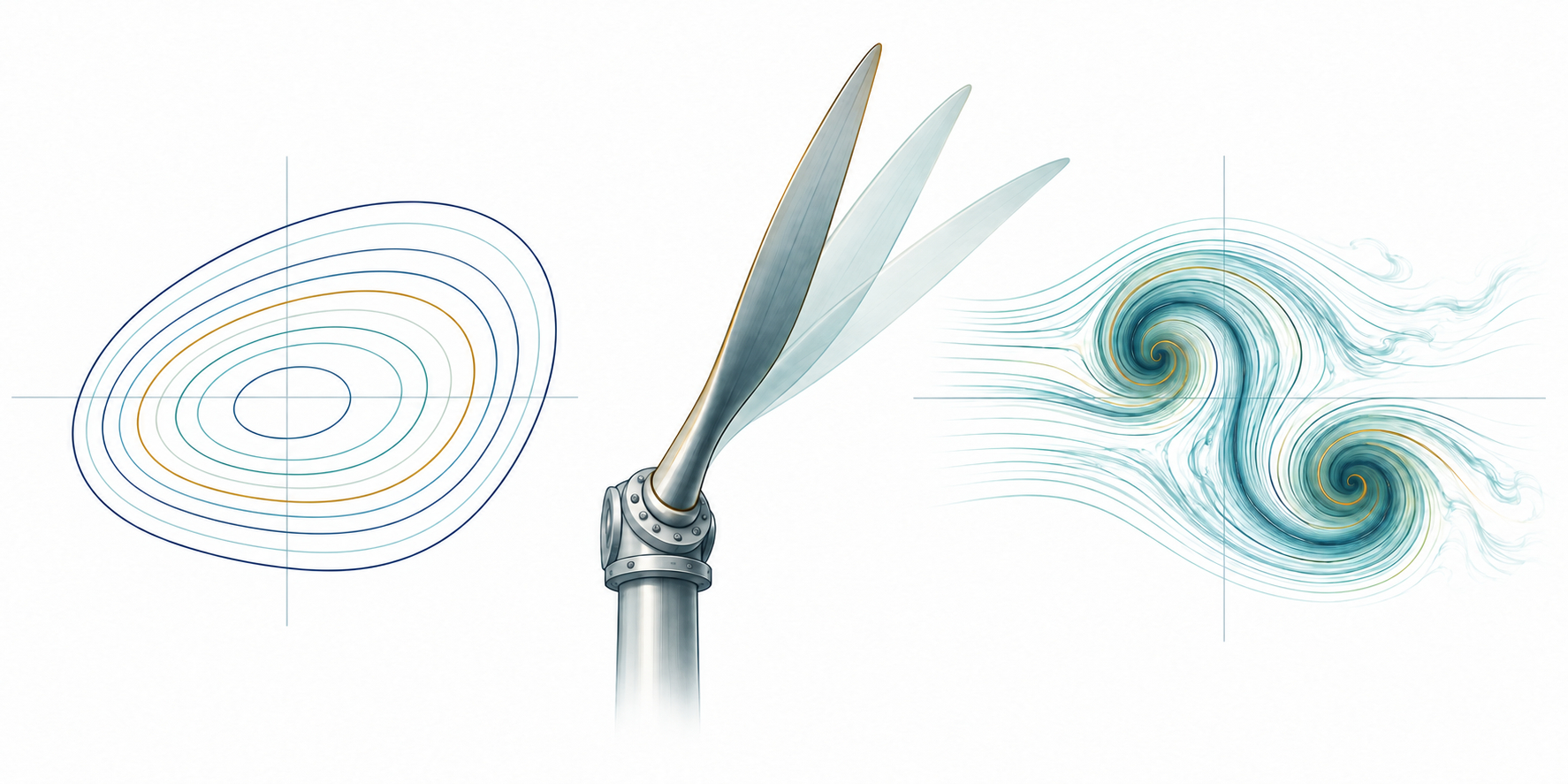
Conceptual illustration of oscillatory motion, a flexible blade, and swirling flow. — An oscillator moves through time, a blade bends along its span, and a fluid flows through a spatial domain. We shall describe these responses through the same construction of fields, relations, and a Lagrangian.

Describing the blade’s motion

Let us consider observing a point on the blade as it goes through bending. We identify the observed point by its position coordinate \(x\) along the undeformed span and observe it at an instant \(t\). These are the coordinates with which we describe where and when the motion occurs. We write the transverse displacement as \(w(x,t)\), and its value tells us how far that point has moved in the transverse direction at that span-wise location and time instant.

To check whether a thickness distribution satisfies the blade’s motion and stress requirements, we need this displacement at every span position and time instant under consideration. Its variation along the span gives the bending deformation, from which we can determine the bending stresses using the material relations. Such an assignment of a value to each point of a domain is what we call a field. The displacement \(w\) is a field; \(w(x,t)\) is its value at the coordinates we have specified.

Suppose the blade has length \(\ell\) and we follow its motion until time \(T\). The span is \(B = [0,\ell]\) and the time interval is \(I = [0,T].\) All pairs \((x,t)\) form the domain \(\mathcal{M} = B \otimes I\) on which the displacement field is defined and observed. Here, \(\otimes\) denotes the product of coordinate domains, whose points are these ordered pairs. These spatio-temporal intervals and their product are examples of manifolds: domains with a smooth local coordinate description, including boundary faces here. For \(B \otimes I\), these include each blade end through time and the span at the initial instant. Specifying the manifold tells us where a field is defined; choosing coordinates lets us label its points.

Now, let us consider the rotation of the rigid hub \(\mathcal{H}\) to which the flexible blade \(\mathcal{B}\) is attached. The hub’s angle \(\varphi(t)\) depends on time alone, so its domain is \(I\). The blade displacement and hub angle describe parts of the same physical system, yet they require different coordinate arguments. To determine their coupled motion, we must relate the blade’s displacement and orientation at its root to the hub’s rotation, and account for the forces and moments transmitted through their attachment. We need to preserve each field’s coordinate dependence when forming these coupling relations.

We shall use the same notation for displacement, hub angle, and the other quantities needed to determine the motion. A field on a manifold \(\mathcal{M}\) is a map

u:\mathcal{M}\longrightarrow\mathbb{R}^{m}, \qquad y\longmapsto u(y).

Here, y denotes the local coordinates and m is the number of components assigned at each point. For the transverse displacement, y = (x,t) and m = 1. For the hub angle, y = t and m = 1. A displacement with several components uses the corresponding vector of values. We collect the unknown fields describing the physical response in Q, which we call the state, while retaining the domain and coordinate arguments of each field.

To express the hub rotation in a blade equation at a span position and time instant (x,t), we select the time coordinate with the projection πₜ(x,t) = t. The resulting field φ ∘ πₜ has the same value at every span location for a given instant. In the hub’s torque balance, we instead integrate the blade’s distributed torque contribution along the span to obtain a quantity depending on time alone. To impose the root attachment condition, we evaluate the blade displacement at the root; this restriction to a face is called a trace. Projection, integration, and restriction give us the quantities on the domains where the coupling relations must hold.

To determine the blade’s motion under an applied load, we need the acceleration that enters its inertia force. We obtain it by differentiating displacement twice with respect to time at a fixed span position. If we give velocity its own field v(x,t), we require v = ∂w/∂t. If we give acceleration its own field a(x,t), we require a = ∂v/∂t. These relations keep the three fields consistent with one motion. We use the word law for a relation that the fields are required to satisfy. Here, the laws specify how one field represents a derivative of another.

More generally, if we retain a field vₖ for the derivative of u along yₖ, we require their difference to vanish:

r_k=\frac{\partial u}{\partial y_k}-v_k=0 \qquad\text{on }\mathcal{M}.

The expression rₖ measures the departure from the required relation; we call it a residual. Setting it to zero imposes the representation law. For a second derivative, we repeat the construction with the derivative of the preceding field. The collection of a field and its derivatives to a specified order is its jet. When we retain these derivatives as separate fields, their representation laws connect them to the same underlying motion. With sufficient smoothness, mixed derivatives must also agree.

To determine the bending moment and stresses during motion, we also need how displacement varies along the span at a fixed instant. Its first span-wise derivative gives the bending slope; for small slopes, the derivative of that slope gives the bending curvature. Curvature enters the bending moment through the stiffness of the blade. We can retain slope and curvature as fields and connect them to displacement through the same derivative laws. Differentiation along time gives velocity; differentiation along the span gives slope. We are applying the same mathematical operation to different coordinates, with a different physical meaning in each case.

Choosing the relations that must hold

The derivative relations connect displacement to velocity, acceleration, slope, and curvature. To determine the motion under a prescribed load, we also need force balance, the starting displacement and velocity, and the conditions at the blade’s attachments. Suppose we hold its thickness at a prescribed distribution while examining that motion. This too is a relation that must hold. We shall state each requirement in the same form: an expression whose value must vanish wherever that requirement applies.

r_a[Q,s](y)=0, \qquad y\in D_a.

The index a names the law, Dₐ is the domain on which it must hold, and s denotes the field or parameters whose influence we want to examine, such as thickness. The residual rₐ[Q,s] is an expression formed from the fields; its value changes as those fields change. Brackets indicate dependence on whole fields through derivatives, traces, or integrals; y specifies where the expression is evaluated. The prescribed information in a relation is its datum: for example, the applied load in force balance or the starting displacement in an initial condition. Physical laws, derivative relations, and prescribed values can all enter through this residual form.

To assess one particular blade design, we need its thickness to remain at the prescribed distribution s₀. We impose rₛ = s − s₀ = 0 and call this relation a pin: it holds a field to its datum. To prescribe the starting displacement, we impose the same relation on the initial face. More generally, \(u\rvert_\Gamma - u_0 = 0\) pins the trace of u on a face Γ. The subscript zero identifies the prescribed value, and the face specifies where we require it.

Suppose we want the blade to follow a target motion. We can measure its departure from that target over the span and time interval, obtaining one number from the displacement field. We denote a scalar quantity formed from the fields by J[Q,s]. It is a functional, and we choose it as the objective when it expresses what we want to assess or improve.

We now want the scalar’s stationarity to enforce the relations that determine an admissible blade motion. How can we make a derivative of the scalar return a required residual? For each residual rₐ, we introduce an unknown multiplier λₐ and pair it linearly with that residual. Variation in λₐ then gives the requirement rₐ = 0. We accumulate the paired contribution over the domain where the law holds. When this pairing can be written as an integral, it takes the form

\begin{aligned} &\langle\lambda_a,r_a\rangle_{D_a}\\ &\qquad=\int_{D_a}\lambda_a(y)\cdot r_a(y)\,d\mu_a(y). \end{aligned}

The measure μₐ specifies how contributions are accumulated over the law’s domain. The multiplier has the corresponding components and coordinate dependence. A law along a span through time has a multiplier of space and time; an initial condition has a multiplier on the initial face. On a single point, the pairing becomes a scalar or dot product. More generally, the multiplier belongs to the dual of the residual space: it acts linearly on a residual to produce a scalar. We choose its units so that the complete paired term has the units of J.

The scalar we construct is

\begin{aligned} \mathcal L[Q,s,\lambda] &=J[Q,s]\\ &\quad+\sum_a\langle\lambda_a,r_a[Q,s]\rangle_{D_a}. \end{aligned}

We place the physical laws, derivative relations, and pins in the same sum. Each contributes a scalar through its own domain pairing. The target-motion objective measures the departure we want to reduce, while the paired relations impose the requirements that the blade’s motion and prescribed thickness must satisfy. Their roles follow from how we use these expressions in the Lagrangian.

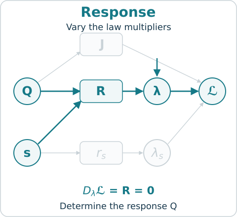
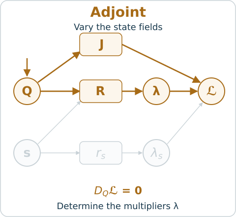
Consider varying the multiplier of any imposed equality. Requiring the first-order change of the scalar to vanish gives that law. Varying the fields gives the equations determining its multipliers. With J = 0, variation in the multipliers still gives the physical laws. Once these determine the response, zero multipliers satisfy stationarity in the state. By adding an objective, we ask how that response affects a quantity of interest.

Reading a multiplier as a sensitivity

Suppose we have determined the blade’s motion for a prescribed material thickness distribution. To improve that distribution, we need the rate at which the motion and stresses change with thickness. Consider describing the distribution by a finite set of design parameters s. As we vary these parameters, the physical laws determine a family of responses. We write Qˢ for the state fields at one design, with components qᵢˢ(yᵢ) on their respective manifolds. Equivalently, qᵢ(yᵢ;s) describes the field over its coordinates and design parameters. Holding s fixed selects the response of one blade design.

We evaluate the objective after determining the physical response and write j(s) = J[Qˢ,s]. This is the reduced objective: the state has been determined by the laws, leaving the design parameters as its arguments. For the blade, a time derivative measures how displacement changes during motion at a fixed design. A design derivative measures how that displacement changes when we alter the thickness distribution. On a fixed domain, we compare these designs at the same span position and instant, holding the coordinates yᵢ fixed.

Let R collect the laws determining Q, including the derivative relations and the initial and boundary conditions. We shall assume that the laws and objective are continuously differentiable. The linearization D_QR of the response laws describes the first-order change in their residuals caused by a change in the state. If this operator is invertible between the chosen state and residual spaces, the field change δQ caused by a parameter change δs satisfies

\begin{aligned} D_QR[\delta Q]&=-D_sR[\delta s],\\ \delta j&=D_QJ[\delta Q]\\ &\quad+D_sJ[\delta s]. \end{aligned}

The symbol D denotes a derivative acting on the indicated variation; a subscript names the argument being varied. The first equation requires the perturbed state to continue satisfying the physical laws to first order. Solving it gives the state change δQ for the chosen design change δs. This is the direct sensitivity. Suppose our design decision requires only the resulting change in the scalar objective. We can eliminate δQ from the objective derivative by choosing multipliers that cancel its contribution. These are precisely the multipliers determined by stationarity in Q:

\begin{aligned} (D_QR)^*\lambda&=-D_QJ,\\ Dj&=D_sJ+(D_sR)^*\lambda. \end{aligned}

The star denotes the dual operator under the chosen pairings. We call the first equation the adjoint equation. The second combines the objective’s explicit dependence on thickness with the contribution caused by the changing motion. It gives the complete first-order change in the objective for any δs, without requiring a separate state sensitivity for each design direction. Once we choose an inner product, we can represent this derivative as a gradient. In either form, the displacement and its adjoint retain their dependence on span position and time.

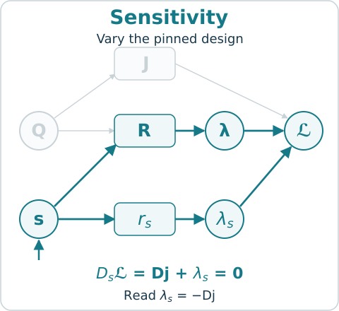
To obtain this objective sensitivity at a particular thickness distribution, we prescribe the design parameters as s₀. We include the design pin and its multiplier:

\mathcal L_{\mathrm{pin}} =\mathcal L+\langle\lambda_s,s-s_0\rangle_{D_s}.

Here, ℒ contains the response laws but not this pin, and Dₛ is the domain of the field s. For finitely many design parameters, we regard s as a vector on a point, so this pairing is a dot product. Stationarity in λₛ fixes s = s₀. After the response and adjoint equations hold, stationarity in s gives Dj + λₛ = 0. Thus the negative of the pin’s multiplier is the sensitivity to its datum. The condition that holds the design also tells us how the objective responds when we change that design! If s is a thickness field, the same statement gives a functional sensitivity distributed over its span.

Suppose we also want to know how the objective changes when we alter a prescribed load or starting displacement. We perturb the datum of the corresponding law by a field εₐ, replacing rₐ = 0 by rₐ − εₐ = 0. If the stationary solution varies differentiably with this datum, and the datum enters only through that law, then

\delta j_*=-\langle\lambda_a,\delta\varepsilon_a\rangle_{D_a}.

Here, j⋆ is the metric evaluated at that stationary solution. To obtain this relation, we differentiate the Lagrangian along the stationary solution. The terms caused by changes in the unknown fields vanish because their stationarity equations hold. What remains is the explicit change in the prescribed datum. The minus sign follows from adding each residual with its multiplier. The pairing matters too: multiplying a law by a nonzero constant divides its multiplier by that constant. Initial data, boundary data, sources, and prescribed designs can all be examined in this way.

Changing what is prescribed

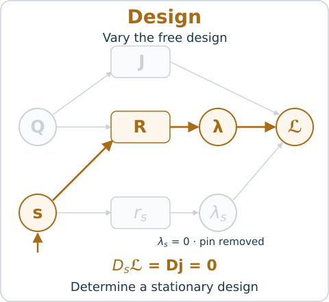
Now suppose we want to choose a thickness distribution that minimizes the objective cost. We remove the design pin term and its multiplier from the Lagrangian, while retaining the laws that determine the blade’s motion. The stationarity equation in s loses the contribution λₛ and becomes Dj = 0. It now determines a candidate design. At an unconstrained interior minimum this condition is necessary; to establish a local minimum, we also examine the objective’s curvature with respect to the design parameters.

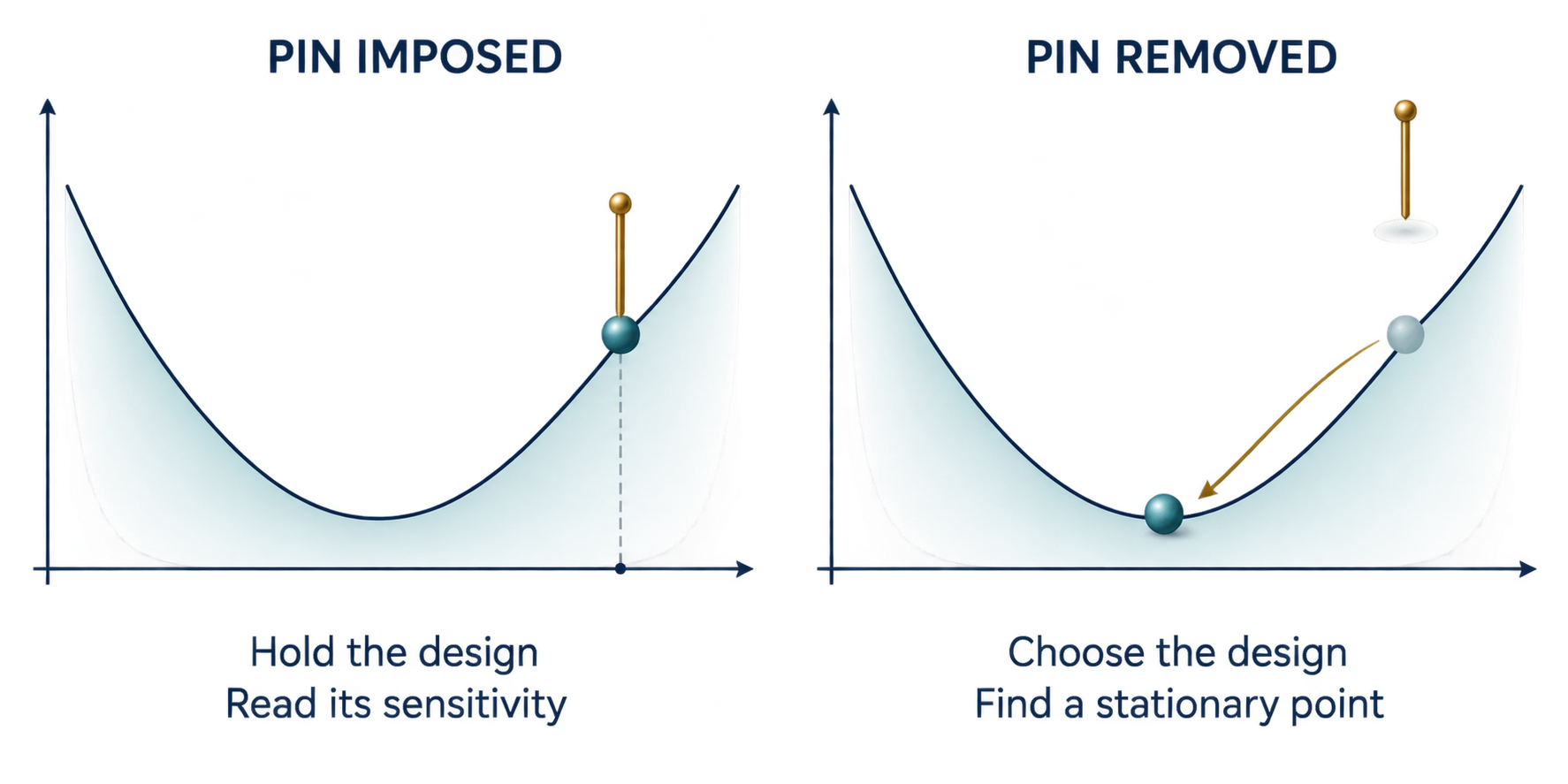
Pin imposed: a design is held away from the objective minimum to read its sensitivity. — We hold a design to read its sensitivity, or release its pin to seek a stationary design. The curve illustrates the reduced objective j(s); the full Lagrangian also contains the physical laws and their multipliers.

Pin removed: the same objective curve, with the design free to seek a stationary point. — We hold a design to read its sensitivity, or release its pin to seek a stationary design. The curve illustrates the reduced objective j(s); the full Lagrangian also contains the physical laws and their multipliers.

We call a field given when its pin is imposed and free when that pin is removed. Other laws can still constrain a free field. A prescribed constant is a given field whose pin has already been substituted. Keeping its pin lets us obtain the sensitivity to that constant from the multiplier.

Suppose we require a stress to stay below the material’s allowable value, or prefer a thickness distribution without insisting on it exactly. We need more than the choice of imposing or removing an equality. We can state these requirements by choosing the relation between each residual and its multiplier:

Imposed: we prescribe the residual’s datum and determine its multiplier.
Removed: we set its multiplier to zero and let the remaining equations determine the fields. A prescribed nonzero multiplier instead retains a known contribution to the scalar; in a mechanical pairing, such a contribution can represent an applied load.
Bounded: we require rₐ ≤ 0, a nonnegative multiplier, and zero pairing between the multiplier and residual. For scalar fields with pointwise multipliers, this reads λₐrₐ = 0 at each point.
Softened: we permit departure from the datum and penalize that departure, with the multiplier determined by λₐ = Wₐrₐ for a specified positive operator Wₐ.

Consider limiting the stress experienced at each span position and time instant. We form the residual as experienced stress minus allowable stress. A negative residual means that the stress is below the limit, and its inequality multiplier is zero. A zero residual means that the limit is active and its multiplier can contribute to design stationarity. To determine a candidate thickness distribution, we balance the objective derivative against the derivatives of the active limits. For a finite collection of differentiable limits cᵢ(s) ≤ 0, evaluated after determining the physical response, a regular constrained minimum therefore satisfies

\begin{gathered} \nabla_s j+\sum_i\eta_i\nabla_s c_i=0,\\ c_i\leq0,\qquad\eta_i\geq0,\\ \eta_i c_i=0. \end{gathered}

The first equation balances the objective derivative against the contributions from the active constraints; the remaining equations enforce the limits and their multiplier conditions. The gradients represent derivatives with respect to the design parameters after the physical response has been determined. Pointwise stress or thickness limits use the corresponding dual conditions on their own domains. Suppose we now want the rate at which the optimal thickness changes with an allowable stress. We need the stationary solution to vary differentiably with that datum. For smooth finite-dimensional problems, independent active-constraint gradients, second-order sufficiency, and strict complementarity provide this locally. If a bound becomes active or inactive, we must examine that change before continuing the derivative argument.

Now suppose we want to penalize departure from a preferred thickness distribution whilst allowing that departure to improve the motion objective. We soften the thickness pin. For a general residual rₐ, we achieve this by replacing its paired term with

\langle\lambda_a,r_a\rangle -\frac12\langle\lambda_a,W_a^{-1}\lambda_a\rangle.

Here, we take Wₐ to be symmetric, positive definite, and invertible under the chosen dual pairing. Stationarity in λₐ gives λₐ = Wₐrₐ. Substituting this relation into the scalar leaves the penalty ½⟨Wₐrₐ,rₐ⟩. For the thickness pin, increasing the weight makes departure from the preferred distribution more costly relative to the motion objective. Decreasing it allows the motion objective more influence over the chosen distribution.

These choices determine what question the Lagrangian answers. With thickness pinned, we assess one blade; with thickness free and stress bounded, we seek a design; with the thickness pin softened, we seek a design that also accounts for departure from a preferred distribution. Removing a general relation can release a requirement among several fields, so the remaining equations must still determine the response.

Design, data, and geometry as fields

So far, we have varied material thickness to improve the blade. Let us consider what else we could vary to meet a target motion. If we vary the applied torque as a field of time, we seek a control that produces that motion. If we vary the initial displacement to match observations of the later motion, we infer the starting state. If we vary a bounded material-density field over a fixed spatial domain, we choose where to place material. In each case, we prescribe a different field or leave it free, pair the required laws with their multipliers, and impose stationarity. The field we vary, its domain, and the objective specify which problem we are solving.

Suppose we also want to vary the blade’s span or the duration of its motion. The displacement fields would then be defined on different spatial or temporal intervals. To differentiate these responses with respect to geometry or duration, we need a common set of reference coordinates at which to compare them. We therefore describe physical positions and instants by maps x(ξ) and t(τ) from fixed reference coordinates ξ and τ. These maps are themselves fields; their values specify where and when a reference point is observed in the physical problem. The pins x − x₀ = 0 and t − t₀ = 0 prescribe the maps. We express the response on the reference domain and apply the chain rule to its physical derivatives. In one spatial dimension,

\begin{aligned} \widehat u(\xi,\tau)&=u(x(\xi),t(\tau)),\\ \frac{\partial u}{\partial t}\circ(x,t) &=\frac{\partial\widehat u/\partial\tau}{\partial t/\partial\tau},\\ \frac{\partial u}{\partial x}\circ(x,t) &=\frac{\partial\widehat u/\partial\xi}{\partial x/\partial\xi}. \end{aligned}

We assume these maps are smooth and invertible, with positive coordinate derivatives. The integration measure transforms as well: dx dt = (∂x/∂ξ)(∂t/∂τ) dξ dτ. A change in span or duration therefore changes both the physical derivatives and the accumulated objective. We retain these dependencies when varying the maps at fixed reference coordinates. Releasing a boundary-position pin permits a geometry change; releasing the final-time pin permits a choice of duration. The transformed laws still constrain each choice. These are smooth variations on a fixed reference manifold; a change in its topology requires an additional construction.

The same construction at successive levels

We have required the blade to satisfy its motion equations while choosing a thickness distribution. Now suppose those motion equations were themselves obtained by requiring a mechanical action to be stationary. To assess or improve that motion, we need the new Lagrangian to retain all the equations obtained from the first. We collect the first level’s fields and multipliers in z, and write its stationarity equations as F[z,s] = 0, with s held as an argument. Pairing these equations with new multipliers μ allows us to introduce a new objective J₁ while preserving the lower level’s stationary response:

\begin{aligned} F[z,s]&=D_z\mathcal L_0[z;s]=0,\\ \mathcal L_1[z,s,\mu] &=J_1[z,s]+\langle\mu,F[z,s]\rangle. \end{aligned}

The pairing here sums over the domains and components of the lower level’s equations. Variation in μ recovers those equations; variation in z determines the new multipliers from the dependence of J₁ on the lower response. We add the new level’s pins and limits in the same manner. The lower level’s physical multipliers now form part of the state, while μ supplies sensitivities of the new objective to perturbations of the lower equations. This is the recurrence we recognize: the equations we derive to determine motion become the laws we impose to improve that motion.

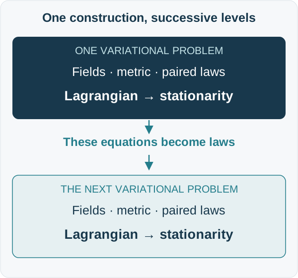
The construction fields, paired laws, Lagrangian, and stationarity repeats at two levels. The first level's stationarity equations become laws of the next level. — We reuse the construction by making one level's stationarity equations laws of the next.

We can repeat this construction whenever a new objective depends on a response already determined by stationarity. At each level, we specify the fields, their domains, the objective, and the laws; variation in the multipliers enforces those laws, and variation in the fields determines their objective sensitivities. For a smooth family of stationary solutions with an invertible linearization, differentiating the objective through the response and reading its negative pin multiplier must give the same derivative. We can use this identity to check the sensitivity derived at each level.

One system and its higher derivatives

At a stationary design, the first derivative of an unconstrained objective vanishes. To determine whether nearby thickness changes increase or decrease the cost, we need its second derivative with respect to those changes. We obtain it by differentiating the same family of stationary solutions again. For sufficiently smooth laws, differentiating the tangent equation gives higher state sensitivities; differentiating the adjoint equation gives the corresponding changes in its multipliers. At each order, the new state derivative appears under the same operator D_QR. The new multiplier derivative appears under its adjoint, with the lower-order derivatives supplying the other terms.

For a scalar prescribed parameter s₀, the pin multiplier along this family therefore satisfies

\frac{d^k j}{ds_0^k} =-\frac{d^{k-1}\lambda_s}{ds_0^{k-1}}, \qquad k\geq1,

provided the required derivatives exist. In particular, the rate at which the negative pin multiplier changes with thickness gives the objective’s curvature with respect to thickness. For several parameters, directional and mixed derivatives follow by differentiating along the corresponding directions. At each order, we differentiate the response to a design change while retaining its span position and time arguments.

This also gives us a way to organize sensitivity methods. The direct method differentiates the response laws and follows the change in state. The adjoint method uses stationarity in the state to remove that change from the metric derivative. Finite differences approximate the derivative by comparing nearby responses. We can also retain intermediate relations and pair each with a multiplier; stationarity then carries the chain rule through those individual relations. Substituting them first gives a statement with fewer intermediate fields and the same derivative.

To see how these routes answer the same sensitivity question, we can draw each field, residual, and objective as a node, with an edge recording which quantity an expression depends on. The paired residuals and objective then lead to one scalar, the Lagrangian. This graph lets us follow the terms contributing to each stationarity equation. We shall now use an oscillator to show these dependencies, then add spatial deformation, connected bodies, fluid motion, and uncertain loading.

Nonlinear oscillation: relations along time

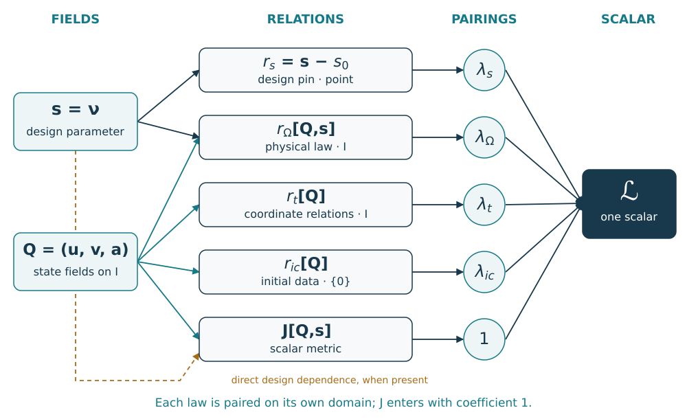
Consider an oscillating displacement whose damping changes with the displacement itself. Suppose we want to determine how the extent of this motion depends on the damping parameter. We shall use the Van der Pol oscillator, with displacement u(t) and damping parameter ν. In this example the quantities are nondimensional. To express the motion law, we retain velocity v(t) and acceleration a(t) as fields on the time interval I = [0, T]. We require the acceleration, damping, and restoring terms to balance, and connect the derivative fields to displacement:

\begin{aligned} r_\Omega&=a-\nu(1-u^2)v+u=0,\\ r_t&=\begin{pmatrix} \partial u/\partial t-v\\ \partial v/\partial t-a \end{pmatrix}=0. \end{aligned}

Substituting the derivative relations for v and a gives the second-order equation in displacement alone. For positive ν, the damping term feeds energy into the motion near equilibrium and removes it at larger displacements. To select the motion we want to assess, we prescribe its starting displacement and velocity through the initial pin r_ic = (u(0) − u₀, v(0) − v₀) = 0 on {0}. The parameter pin rₛ = ν − ν₀ = 0 fixes the damping parameter on a point domain. These pins distinguish one prescribed motion from the family generated by changing the starting data or damping.

Suppose we want to assess the displacement from equilibrium and the speed of motion over this interval. We combine their squared values into the objective

J=\int_0^T\frac{u(t)^2+v(t)^2}{2}\,dt.

We pair rΩ and the two components of rₜ with their own multipliers on I, and pair the pins on their point domains. Stationarity gives the equations determining the motion, the adjoint equations in the three state fields, and the objective sensitivity dj/dν₀ = −λₛ to the prescribed damping parameter. The negative multipliers of the initial pins similarly give the objective sensitivities to the starting displacement u₀ and velocity v₀. Removing the parameter pin lets us seek a stationary value of the same objective by varying ν.

Figure 1. We assemble the oscillator's Lagrangian from its fields and relations. Here, Q = (u, v, a) and s = ν. Each residual is paired with its multiplier on the domain indicated. The dashed edge applies when J depends directly on s; it is absent for the objective used above.

Varying the response-law multipliers returns the laws that determine the state. — **Figure 2.** We read four questions from the same graph by changing what we vary and whether the design pin is present. R collects all response laws, including coordinate relations and initial conditions; λ collects their multipliers. Highlighted paths identify the terms contributing to each variation. Arrows show mathematical dependence. The reduced derivative Dj is read after the response and adjoint equations hold.

Varying the state gives the adjoint equations for the response multipliers. — **Figure 2.** We read four questions from the same graph by changing what we vary and whether the design pin is present. R collects all response laws, including coordinate relations and initial conditions; λ collects their multipliers. Highlighted paths identify the terms contributing to each variation. Arrows show mathematical dependence. The reduced derivative Dj is read after the response and adjoint equations hold.

Beam mechanics: adding a spatial factor

Now consider choosing the stiffness of a beam so that its bending motion follows a prescribed target. We need the acceleration to determine the inertia force and the curvature to determine the bending moment. The oscillator required derivatives along time; bending also requires derivatives along space. The deflection w(x,t) is defined on B ⊗ I. We retain velocity v, acceleration a, slope ψ, and curvature χ on this same manifold, and connect them to deflection through

\begin{aligned} r_t&=\begin{pmatrix} \partial w/\partial t-v\\ \partial v/\partial t-a \end{pmatrix}=0,\\ r_x&=\begin{pmatrix} \partial w/\partial x-\psi\\ \partial\psi/\partial x-\chi \end{pmatrix}=0. \end{aligned}

To determine the deflection under an applied transverse load, we impose force balance. For an undamped Euler–Bernoulli beam, this gives

r_\Omega=\rho A\,a+ \frac{\partial^2(EI\chi)}{\partial x^2}-f=0.

Here, ρA is mass per unit length, EI is the stiffness against bending deformation, and f(x,t) is the applied transverse force per unit length. The bending moment EIχ depends on curvature, and its second span-wise derivative enters the force balance with the inertia term ρAa. Substituting the derivative relations gives a fourth-order spatial and second-order temporal equation for the deflection. We therefore need conditions at the beam ends as well as its starting displacement and velocity to determine the motion.

We pin displacement w and velocity v on B ⊗ {0} to specify the starting motion along the whole span. We also need to state how the beam is supported at its ends. A simply supported end has zero deflection and bending moment; a clamped end has zero deflection and slope. These conditions hold on {0} ⊗ I or {ℓ} ⊗ I, throughout the motion. Each relation has a multiplier on its own domain with the required component structure.

Suppose we want to choose the bending stiffness along the span so that the beam follows a target displacement w⋆(x,t). For this example, we vary stiffness while holding the mass per unit length and applied load fixed. We choose a family of positive stiffness distributions,

\begin{gathered} EI(x;s)=EI_0\left(1+s_1\xi+s_2\xi^2\right),\\ \xi=x/\ell, \end{gathered}

and use the squared departure from the target displacement as the objective cost,

\begin{aligned} J&=\frac12\int_0^T\!\int_0^\ell\\ &\qquad\bigl(w(x,t)-w_\star(x,t)\bigr)^2\,dx\,dt. \end{aligned}

The parameters s₁ and s₂ control the linear and quadratic variation of stiffness along the span. Each choice gives a displacement w(x,t;s) and its associated derivative fields. Pinning the two parameters gives two objective sensitivities. Removing those pins lets us seek a stiffness distribution that reduces the departure from the target motion, subject to positive bending stiffness along the beam.

Now suppose the same beam must serve under two different applied loads. We give each load case its own displacement, derivative fields, physical laws, and multipliers, while retaining one stiffness design s. We sum the two objective costs and their paired laws, and include the shared design pin once. Stationarity in s then combines the effects of both load cases on the design decision. One beam design must accommodate both motions.

Connected bodies: nesting variational problems

Suppose we now connect several bodies and want to determine how changing one body’s inertia affects the motion of another. We must account for the forces transmitted through their joints while requiring their attachment points to remain together. Consider a triple pendulum, with positions and orientations q(t) varying through time. The relations gᵦ(q,t,s) = 0 express the required joint connections. To obtain the motion equations and joint reactions together, we pair these relations with multipliers ηᵦ in the mechanical action

\begin{aligned} \mathcal A=\int_0^T\!\Bigl(&K(q,\dot q,s)-V(q,s)\\ &+\sum_b\eta_b\cdot g_b(q,t,s)\Bigr)\,dt. \end{aligned}

Here, K and V are kinetic and potential energy, and the joint multipliers ηᵦ are fields of time. Variation in ηᵦ returns the joint conditions. Variation in q, with variations vanishing at the temporal endpoints, gives the motion equations with joint reactions. Initial positions and velocities consistent with the joints select the trajectory.

Suppose we want to know how the last body’s vertical motion changes with the first body’s inertia. We can measure the last body’s displacement from its initial height, integrate its square over time, and take this as J. The motion equations and joint conditions now enter the sensitivity Lagrangian as laws. The physical joint reactions belong to the response being determined, while the new multipliers measure the objective’s sensitivity to perturbations of these laws. We have used stationarity to obtain the motion equations, and now use those equations to obtain a design derivative.

Let us now return to the flexible blade \(\mathcal{B}\) attached to the rigid hub \(\mathcal{H}\). To determine how a thickness change affects their coupled motion, we need both the blade’s deformation along its span and the hub’s rotation through time. If m(x,t) is the blade’s torque contribution per unit span, then ∫_B m(x,t) dx is the total distributed contribution entering the hub’s torque balance. The root attachment conditions require compatibility of the blade’s root displacement and orientation with the hub motion. Their multipliers supply the attachment forces and moments in the mechanical equations. We form each coupling relation on its own domain before pairing it with a multiplier.

We can now state the original thickness question in terms of these fields and laws. For a specified material and cross-sectional form, the smooth span-wise thickness field h(x) determines the area and stiffness, which affect the motion and the stresses experienced during it. To assess a prescribed distribution h₀(x), we include the pin h − h₀ = 0 and choose a metric of interest, such as blade mass or a measure of stress during motion. The negative pin multiplier gives the rate at which that metric changes with the span-wise thickness distribution.

Suppose our target is the least mass that can carry the required loads. We choose the objective by integrating density times area along each blade. We include the motion and joint laws as equalities, and thickness and stress limits as inequalities on their respective domains. We leave the thickness unpinned. Stationarity now determines a candidate distribution, with the active limits contributing through their own multipliers. Each term in the scalar has a job in choosing the blade.

If the blades must operate under collective and cyclic control, each prescribed operating case has its own motion and laws. The blade must meet the motion and strength requirements in all of these cases with one material thickness distribution. Each case therefore contributes to stationarity in the shared thickness field. We have extended the design question across operating conditions while retaining the same construction of the Lagrangian.

Fluid motion: coupled fields and a pressure condition

The blade and hub required coupling between fields on different manifolds. Let us now consider velocity and pressure on the same manifold, and ask how viscosity affects the persistence of an incompressible swirling flow such as the Taylor–Green vortex. We need the velocity to measure the motion and the pressure to enforce the requirement that the fluid preserve volume. The spatial manifold B is periodic, and the velocity u(x,t) and kinematic pressure p(x,t) are fields on B ⊗ I. For constant density, we impose momentum balance and volume conservation:

\begin{gathered} \partial_t\mathbf u +(\mathbf u\cdot\nabla)\mathbf u +\nabla p-\nu\Delta\mathbf u=0,\\ \nabla\cdot\mathbf u=0. \end{gathered}

The first equation balances fluid acceleration against pressure and viscous effects; the second requires the velocity field to preserve volume locally. Here, ν is kinematic viscosity, and p is pressure divided by density. To represent how velocity varies with spatial position, we can retain its gradient components Gᵢⱼ as separate fields. We then include ∂uᵢ/∂xⱼ − Gᵢⱼ = 0 on the space-time domain. The initial velocity is pinned on B ⊗ {0}. These derivative relations and their multipliers enter the scalar as they did for beam displacement and slope.

To obtain a sensitivity from the response equations, we first need to remove any freedom that leaves the physical response unchanged. Suppose we add a spatially uniform value to pressure at each instant. Its spatial gradient remains unchanged, so the motion equations cannot determine that pressure level. We fix it by prescribing zero spatial mean pressure:

\int_B p(\mathbf x,t)\,d\mathbf x=0 \qquad\text{for each }t.

The pressure condition and its multiplier live on I, while pressure lives on B ⊗ I. This is another instance of spatial integration producing a field of time. Specifying the integrand, domain, and measure gives the shared operation its physical meaning. It also exposes a requirement for the sensitivity argument: an undetermined pressure level must be fixed before we can assume an invertible response linearization.

Suppose we want to assess how much swirling motion persists over the time interval. We integrate the squared fluid speed over space and time to form the objective

J=\frac12\int_0^T\!\int_B \mathbf u\cdot\mathbf u\,d\mathbf x\,dt.

We pair the momentum, volume-conservation, derivative, initial-velocity, and pressure conditions with their multipliers. A viscosity pin ν − ν₀ = 0 then lets us obtain the rate at which this measure of fluid motion changes with viscosity. We have changed the physical response and the objective used to assess it; the pin multiplier still gives the objective derivative through stationarity.

Extending the construction to probabilistic space-time

Suppose the applied load is uncertain, so that one beam design must accommodate a range of possible motions. To choose a thickness distribution under this uncertainty, we need to assess both the motion under each possible load and how probable that load is. We describe the uncertain load by parameters θ, with possible values in Θ and a prescribed probability density pΘ. The displacement is now w(θ,x,t;s): its value specifies the transverse displacement at a load realization θ, span position x, and time instant t, for the shared design s. These arguments give the domain Θ ⊗ B ⊗ I. We shall carry the field, derivative, and pairing constructions across this probabilistic space-time (PST) domain.

To enforce the motion law for each possible load, we give it a multiplier depending on θ, space, and time; an initial condition retains θ and space. Every represented derivative likewise retains the coordinate dependence of the field it describes. Suppose we need the rate at which displacement changes with an uncertain load parameter θₖ. Where the response is differentiable in θₖ, we retain that derivative as a field and impose its representation law, holding span position, time, and design fixed. We are using the same derivative relation as for span position and time, now to describe dependence on the applied load. This is the common structure we seek in PST mathematics.

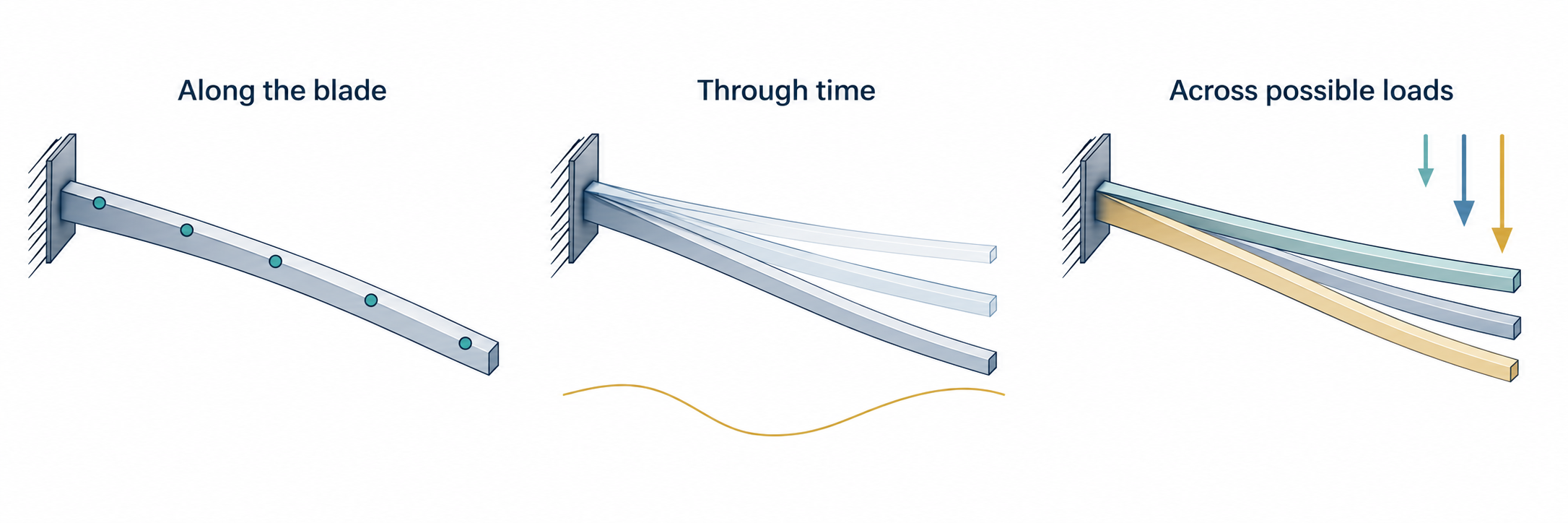
Along the blade: the response depends on position along its span. — We describe the blade's displacement along its span, through its motion, and across possible applied loads. Each coordinate identifies a dependence of the displacement field; the material thickness distribution is shared across these cases.

Through time: successive blade positions show its motion. — We describe the blade's displacement along its span, through its motion, and across possible applied loads. Each coordinate identifies a dependence of the displacement field; the material thickness distribution is shared across these cases.

We are choosing one blade to operate under the uncertain load. Its material thickness h(x) varies along the span and stays fixed whilst the blade moves under each possible load. To evaluate it in a motion law at (θ,x,t), we select the span coordinate by projection onto B and use the value h(x). We used the same operation to evaluate the hub angle in a blade equation. Allowing a separate h(θ,x) would ask a different design question: the thickness could then change with the realized load.

For each possible load θ, we first evaluate the objective over the span and time interval after determining the motion. This gives j(θ;s), the objective cost for that load and design. To assess the design across uncertain loads, we need to combine these costs according to their probability distribution. For square-integrable scalar fields on Θ, we use the weighted pairing

\begin{aligned} &\langle f,g\rangle_{p_\Theta}\\ &\qquad=\int_\Theta f(\theta)g(\theta)p_\Theta(\theta)\,d\theta. \end{aligned}

Expectation is another integral, with the probability density supplying its weight! We have already accumulated contributions over span and time; we now accumulate them across the uncertain loads. Pairing the objective with one gives its mean cost, while pairing its departure from the mean with itself gives its variance:

\begin{aligned} m(s)&=\langle j,1\rangle_{p_\Theta},\\ v(s)&=\langle j-m,j-m\rangle_{p_\Theta}. \end{aligned}

We can therefore choose m + βv, with β ≥ 0, as the objective cost to minimize. The weight β specifies how much we penalize variation in cost across possible loads in addition to its mean. We choose its units so that both terms have the same units. To construct the Lagrangian before determining the motion, we form the mean M and variance V from the objectives J[Q(θ),s] in terms of the unknown response fields. We then add the expectation of the paired motion and data relations, together with the shared design pin:

\begin{gathered} \mathcal L_U=M+\beta V\\ \quad+\mathbb E_\theta\!\left[\sum_a \langle\lambda_a,r_a\rangle_{D_a}\right]\\ \quad+\langle\lambda_s,s-s_0\rangle_{D_s}. \end{gathered}

Inside the expectation, each residual and multiplier depends on θ. Each load case contributes its laws over the required physical domains, and the expectation supplies the probability weighting. The shared pin is paired once over the design field’s own domain. Stationarity determines the motion and adjoint fields across possible loads, and combines their contributions in the shared design equation. Once the physical laws hold, M = m(s) and V = v(s). The negative design-pin multiplier therefore gives the sensitivity of m + βv to the prescribed design; removing that pin lets us seek a stationary design for the statistical objective.

To improve the shared thickness distribution, we need the rates at which both the mean cost and its variance change with that distribution. If the probability density is independent of the design and differentiation under the expectation is justified, these reduced derivatives are

\begin{aligned} Dm&=\mathbb E[Dj],\\ Dv&=2\mathbb E[(j-m)Dj]. \end{aligned}

The second relation uses 𝔼[j − m] = 0. The derivative Dj at each θ comes from the motion laws, derivative relations, and adjoint construction for that load. The mean derivative weights these sensitivities by probability; the variance derivative also weights them by the departure of each cost from the mean. These are the contributions we combine when choosing a thickness distribution to reduce the statistical objective.

Our choice of scalar is therefore a design decision in its own right. To assess a prescribed blade, we include its material thickness pin and read the chosen metric’s design sensitivity. To seek a lighter blade, we choose mass as the objective and vary the span-wise thickness subject to the motion and strength requirements. To account for uncertain loading, we choose a statistical objective and combine the possible responses through probability-weighted pairings. We engineer the Lagrangian by choosing what to vary and which relations to impose, so that stationarity gives the outcome we seek subject to the stated constraints.

Share on

Twitter Facebook LinkedIn

Komahan Boopathy